Next: Visualization of the Wavelet
Up: Multiresolution with scaling functions
Previous: The Wavelet transform using
If the wavelet is the difference between two resolutions,
an evident reconstruction for a wavelet transform
 is:
is:
 |
|
|
(14.60) |
But this is a particular case and other wavelet functions can be
chosen. The reconstruction can be done step by step, starting from
the lowest resolution. At each scale, we have the relations:
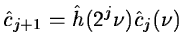 |
|
|
(14.61) |
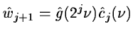 |
|
|
(14.62) |
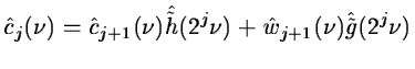
we look for cj knowing cj+1, wj+1, h and g.
We restore
 with a least mean square estimator:
 |
|
|
(14.63) |
is minimum.
 and
and
 are weight
functions which permit a general solution to the
restoration of
are weight
functions which permit a general solution to the
restoration of
 .
By
.
By
 derivation we get:
 |
|
|
(14.64) |
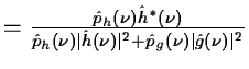
where the conjugate filters have the expression:
It is easy to see that these filters satisfy the exact reconstruction
equation 14.19. In fact, equations
14.65 and 14.66 give the
general solution to this equation. In this analysis, the
Shannon sampling condition is always respected. No aliasing
exists, so that the dealiasing condition 14.18 is not
necessary.
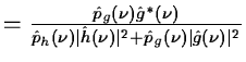
The denominator is reduced if we choose:
This corresponds to the case where the wavelet is the difference between
the square of two resolutions:
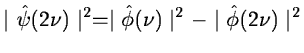 |
|
|
(14.67) |
Figure 14.10:
Left, the interpolation function
 and right, the wavelet
 .
.
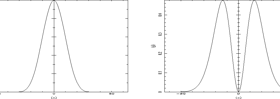 |
Figure:
On left, the filter
 ,
and on right the filter
,
and on right the filter
 .
.
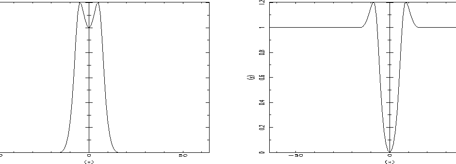 |
We plot in figure 14.10 the chosen scaling function
derived from a B-spline of degree
3 in the frequency space and
its resulting wavelet function. Their
conjugate functions are plotted in figure 14.11.
The reconstruction algorithm is:
- 1.
- We compute the FFT of the image at the low resolution.
- 2.
- We set j to np. We iterate:
- 3.
- We compute the FFT of the wavelet coefficients at the scale j.
- 4.
- We multiply the wavelet coefficients
 by
by
 .
.
- 5.
- We multiply the image at the lower resolution
 by
by
 .
.
- 6.
- The inverse Fourier Transform of the addition of
 and
and
 gives the
image cj-1.
gives the
image cj-1.
- 7.
- j = j - 1 and we go back to 3.
The use of a scaling function with a cut-off frequency
allows a reduction of sampling at each scale, and limits the
computing time and the memory size.
Next: Visualization of the Wavelet
Up: Multiresolution with scaling functions
Previous: The Wavelet transform using
Petra Nass
1999-06-15