Next: The à trous algorithm
Up: The discrete wavelet transform
Previous: Introduction
Multiresolution Analysis
Multiresolution analysis [25] results
from the embedded subsets generated by the interpolations at
different scales.
A function f(x) is projected at each step j onto the subset
Vj. This projection is defined by the scalar product cj(k) of
f(x) with the scaling function  which is dilated and
translated:
which is dilated and
translated:
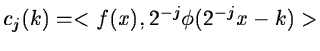 |
|
|
(14.9) |
As  is a scaling function which has the property:
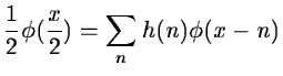 |
|
|
(14.10) |
or
 |
|
|
(14.11) |
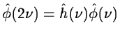
where
 is the Fourier transform of the function
 .
We get:
.
We get:
 |
|
|
(14.12) |
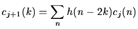
Equation 14.10 permits to
compute directly the set
cj+1(k) from cj(k).
If we start from the set c0(k) we compute all the sets
cj(k), with j>0, without directly computing any other scalar
product:
 |
|
|
(14.13) |
At each step, the number of scalar products is divided by 2. Step by step
the signal is smoothed and information is lost. The remaining
information can be restored using the complementary subspace Wj+1 of
Vj+1 in Vj.
This subspace can be generated by a suitable wavelet function
 with translation and dilation.
 |
|
|
(14.14) |
or
 |
|
|
(14.15) |
We compute the scalar products
 with:
with:
 |
|
|
(14.16) |
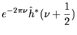
With this analysis, we have built the first part of a filter bank
[34]. In order to restore the original data, Mallat uses
the properties of orthogonal wavelets, but the theory has been
generalized to a large class of filters [8] by introducing two
other filters  and
and  named conjugated to h and
g. The restoration is performed with:
named conjugated to h and
g. The restoration is performed with:
![$\displaystyle c_{j}(k)=2\sum_l [c_{j+1}(l)\tilde h(k+2l)+w_{j+1}(l)\tilde g(k+2l)]$](img618.gif) |
|
|
(14.17) |
In order to get an exact restoration, two conditions are required
for the conjugate filters:
- Dealiasing condition:
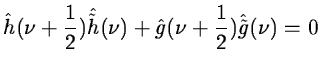 |
|
|
(14.18) |
- Exact restoration:
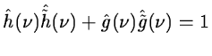 |
|
|
(14.19) |
Figure 14.3:
The filter bank associated with the multiresolution
analysis
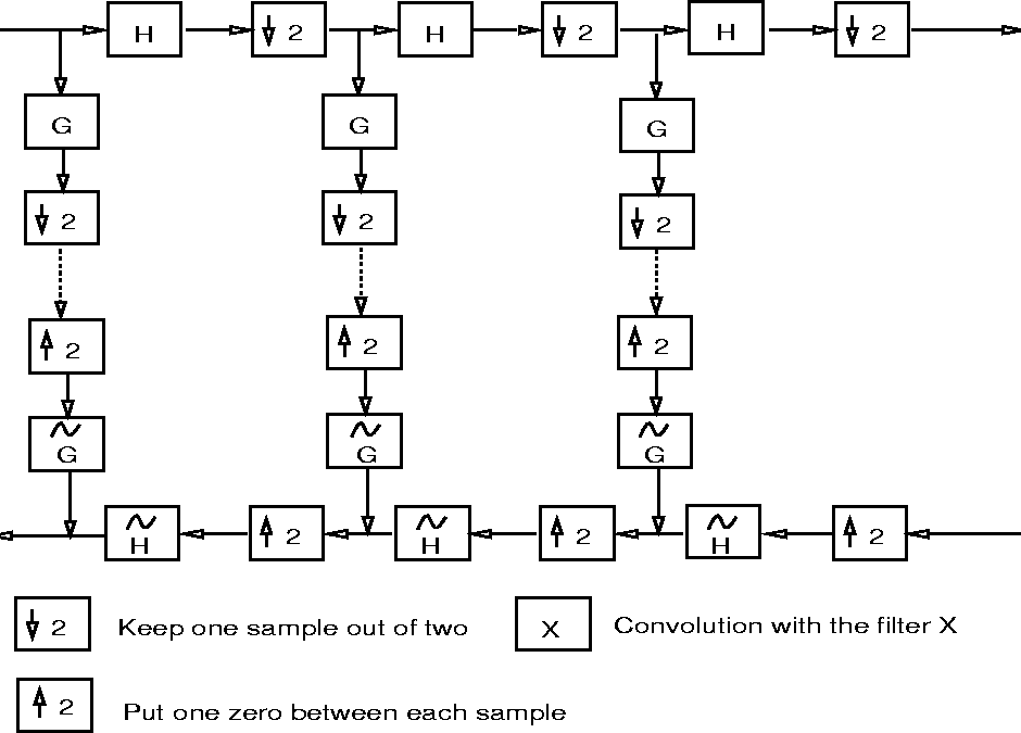 |
In the decomposition, the function is successively convolved with
the two filters H (low frequencies) and G (high frequencies). Each
resulting function is decimated by suppression of one sample out of two. The
high frequency signal is left, and we iterate with the low frequency signal
(upper part of figure 14.3).
In the reconstruction, we restore the sampling by inserting a 0 between
each sample, then we convolve with the conjugate filters  and
and
 ,
we add the resulting functions and we multiply the result by 2.
We iterate up to the smallest scale
(lower part of figure 14.3).
,
we add the resulting functions and we multiply the result by 2.
We iterate up to the smallest scale
(lower part of figure 14.3).
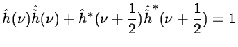
Orthogonal wavelets correspond to the restricted case where:
 |
= |
 |
(14.20) |
 |
= |
 |
(14.21) |
 |
= |
 |
(14.22) |
and
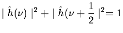 |
|
|
(14.23) |
We can easily see that this set satisfies the two basic
relations 14.18 and 14.19.
Daubechies wavelets are the only compact solutions.
For biorthogonal wavelets [8]
we have the relations:
and
 |
|
|
(14.26) |
We also satisfy relations 14.18 and 14.19. A large class of
compact wavelet functions can be derived.
Many sets of filters were proposed, especially for coding. It was shown
[9] that the choice of these filters must be guided by the
regularity of the scaling and the wavelet functions.
The complexity is proportional to N. The algorithm provides a pyramid of
N elements.
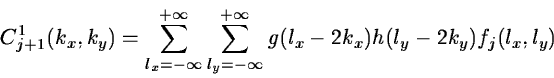
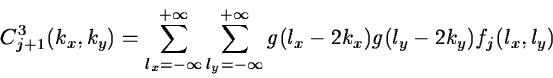
The 2D algorithm is based on separate variables leading to
prioritizing of x and y directions. The scaling function is defined by:
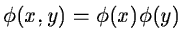 |
|
|
(14.27) |
The passage from a resolution to the next one is done by:
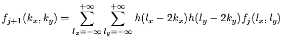 |
|
|
(14.28) |
The detail signal is obtained from three wavelets:
- a vertical wavelet :
- a horizontal wavelet:
- a diagonal wavelet:
which leads to three sub-images:
Figure 14.4:
Wavelet transform representation of an image
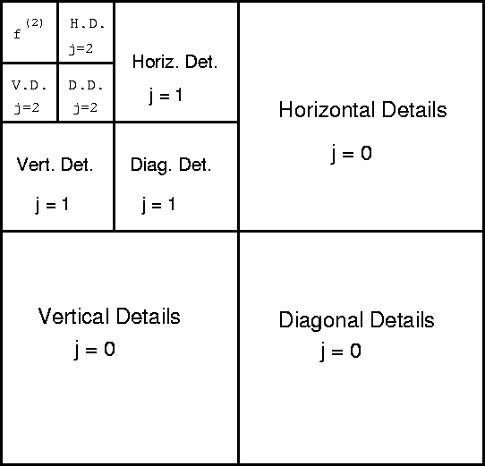 |
The wavelet transform can be interpreted as the decomposition on
frequency sets with a spatial orientation.
Next: The à trous algorithm
Up: The discrete wavelet transform
Previous: Introduction
Petra Nass
1999-06-15