


Next: Geometric Corrections
Up: Raw to Calibrated Data
Previous: Artifacts
The raw data values from the detector system have to be transformed
into relative intensities which then can later be adjusted to an
absolute scale by comparison with standard objects. The majority of
modern detectors (e.g. CCD, diode-array or image tube) have a nearly
linear response while photographic emulsions are strongly non-linear.
Even for the `linear' detectors, a number of corrections must be
included in the intensity calibration. Some of these can be derived
theoretically such as dead-time corrections for photon counting
devices or saturation effects for electronographic emulsions while
other non-linear effects are determined empirically. Systems which
are assumed to be linear need only be corrected for a possible dark
count and bias in addition to the relative sensitivity variation over
the detector. The correction frames are determined from a set of test
exposures from which artifacts are removed first as described in
Section 2.2.1. A raw frame Ci,j is then transformed to
relative intensities Ii,j by
 |
(2.10) |
where Di,j is the appropriate dark counts including bias and
Fi,j is a normalized flat field exposure.
A mathematical function is used to transform data from detectors with
non-linear response to a more linear domain. For photographic
emulsions Baker (1925) found the formula
 |
(2.11) |
which makes the lower part of the characteristic curve almost linear.
In Equation 2.11, D is the photographic density above fog.
These values can then, by means of least squares methods, be fitted
with a power series
 |
(2.12) |
where n for most applications is smaller than 7. The characteristic
curves are shown in Figure 2.4 both using normal and
Backer densities. The coefficients ak depend not only on the
emulsion type but also on the spectral range. For spectral plates
this leads to a positional variation of the terms ak.
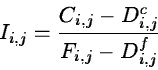
Figure 2.4:
A density-intensity transformation curve for a photographic
emulsion using normal densities (A) and Backer densities (B).
 |
The main problem with non-linear detectors is not so much to
determine the response curve as the modification of the noise
distribution. Thus, the gaussian grain noise on emulsions becomes
skewed through the intensity calibration. Special care must be taken
in the further processing to avoid systematic error due to
non-gaussian noise (e.g. the average of a region will be biased).
One possible way to make the distribution more gaussian again is to
apply a median filter because it is less affected by the
transformation.
Next: Geometric Corrections
Up: Raw to Calibrated Data
Previous: Artifacts
Petra Nass
1999-06-15