

This chapter demonstrates the use of XSPEC. The brief discussion of data and response files is followed by fully worked examples using real data that include all the screen input and output with a variety of plots. The topics covered are as follows: defining models, fitting data, determining errors, fitting more than one set of data simultaneously, simulating data, and producing plots.
Brief Discussion of XSPEC Files
At least two files are necessary for use with XSPEC: a data file and a response file. In some cases, a file containing background may also be used, and, in rare cases, a correction file is needed to adjust the background during fitting. If the response is split between an rmf and an arf then an ancillary response file is also required. However, most of the time the user need only specify the data file, as the names and locations of the correct response and background files should be written in the header of the data file by whatever program created the files.
Fitting Models to Data: An Example from EXOSAT
The 6s X-ray pulsar 1E1048.1–5937 was observed by EXOSAT in June 1985 for 20 ks. In this example, we'll conduct a general investigation of the spectrum from the Medium Energy (ME) instrument, i.e. follow the same sort of steps as the original investigators (Seward, Charles & Smale, 1986). The ME spectrum and corresponding response matrix were obtained from the HEASARC On-line service. Once installed, XSPEC is invoked by typing
%xspec
as in this example:
%xspec
XSPEC version: 12.2.1
Build Date/Time: Wed Nov 2 16:16:52 2005
XSPEC12>data s54405.pha
1 spectrum in use
Source File: s54405.pha
Net count rate (cts/s) for Spectrum:1 3.783 +/- 0.1367
Assigned to Data Group 1 and Plot Group 1
Using Response (RMF) File s54405.rsp
The data command tells the program to read the data as well as the response file that is named in the header of the data file. In general, XSPEC commands can be truncated, provided they remain unambiguous. Since the default extension of a data file is .pha, and the abbreviation of data to the first two letters is unambiguous, the above command can be abbreviated to da s54405, if desired. To obtain help on the data command, or on any other command, type help command followed by the name of the command.
One of the first things most users will want to do at this stage—even before fitting models—is to look at their data. The plotting device should be set first, with the command cpd (change plotting device). Here, we use the pgplot X-Window server, /xw.
XSPEC12> cpd /xw
There are more than 50 different things that can be plotted, all related in some way to the data, the model, the fit and the instrument. To see them, type:
XSPEC12> plot ?
plot data/models/fits etc
Syntax: primary plot commands:
chisq contour counts data delchi
emodel eemodel efficiency eufspec eeufspec
foldmodel icounts insensitivity delchi lcounts
model ratio residuals sensitivity sum
ufspec
secondary options (2-panel data plots - use with data, ldata, counts, lcounts, icounts):
chisq delchi ratio residuals
The most fundamental is the data plotted against instrument channel (data); next most fundamental, and more informative, is the data plotted against channel energy. To do this plot, use the XSPEC command setplot energy. Figure A shows the result of the commands:
XSPEC12> setplot energy
XSPEC12> plot data
Figure A: The result of the command plot data when the data file in question is the EXOSAT ME spectrum of the 6s X-ray pulsar 1E1048.1--5937 available from the HEASARC on-line service
People familiar with EXOSAT ME data will recognize the spectrum to be soft, absorbed and without an obvious bright iron emission line. We are now ready to fit the data with a model. Models in XSPEC are specified using the model command, followed by an algebraic expression of a combination of model components. There are two basic kinds of model components: additive, which represent X-Ray sources of different kinds. After being convolved with the instrument response, the components prescribe the number of counts per energy bin (e.g., a bremsstrahlung continuum); and multiplicative models components, which represent phenomena that modify the observed X-Radiation (e.g. reddening or an absorption edge). They apply an energy-dependent multiplicative factor to the source radiation before the result is convolved with the instrumental response.
More generally, XSPEC allows three types of modifying components: convolutions and mixing models in addition to the multiplicative type. Since there must be a source, there must be least one additive component in a model, but there is no restriction on the number of modifying components. To see what components are available, type model ?:
XSPEC12>model
Additive Models:
apec bbody bbodyrad bexrav bexriv bknpower
bmc bremss c6mekl c6pmekl c6vmekl cemekl
cevmkl cflow compLS compST compTT compbb
cutoffpl disk diskbb diskline diskm disko
diskpn equil gaussian gnei grad grbm
laor lorentz meka mekal mkcflow nei
npshock nteea pegpwrlw pexrav pexriv plcabs
posm powerlaw pshock raymond redge refsch
sedov srcut sresc step vapec vbremss
vequil vgnei vmcflow vmeka vmekal vnei
vnpshock vpshock vraymond vsedov zbbody zbremss
zgauss zpowerlw
Multiplicative Models:
SSS_ice TBabs TBgrain TBvarabs absori cabs
constant cyclabs dust edge expabs expfac
highecut hrefl notch pcfabs phabs plabs
redden smedge spline uvred varabs vphabs
wabs wndabs xion zTBabs zedge zhighect
zpcfabs zphabs zvarabs zvfeabs zvphabs zwabs
zwndabs
Convolution Models:
gsmooth lsmooth reflect
Pile-up Models:
pileup
Additive Models: 68
Multiplicative Models: 37
Convolution Models: 3
Pile-up Models: 1
Total Models: 109
For information about a specific component, type help model followed by the name of the component):
XSPEC12>help model raymond
Given the quality of our data, as shown by the plot, we'll choose an absorbed power law, specified as follows :
XSPEC12> model phabs(powerlaw)
Or, abbreviating unambiguously:
XSPEC12> mo pha(po)
The user is then prompted for the initial values of the parameters. Entering <return> or / in response to a prompt uses the default values. We could also have set all parameters to their default values by entering /* at the first prompt. As well as the parameter values themselves, users also may specify step sizes and ranges (<value>, <delta>, <min>, <bot>, <top>, and <max values>), but here, we'll enter the defaults:
XSPEC12>mo pha(po)
Model: phabs[1]( powerlaw[2] )
Input parameter value, delta, min, bot, top, and max values for ...
Current: 1 0.001 0 0 1E+05 1E+06
phabs:nH>/*
---------------------------------------------------------------------------
---------------------------------------------------------------------------
Model: phabs[1]( powerlaw[2] )
Model Fit Model Component Parameter Unit Value
par par comp
1 1 1 phabs nH 10^22 1.000 +/- 0.
2 2 2 powerlaw PhoIndex 1.000 +/- 0.
3 3 2 powerlaw norm 1.000 +/- 0.
---------------------------------------------------------------------------
---------------------------------------------------------------------------
Chi-Squared = 4.8645994E+08 using 125 PHA bins.
Reduced chi-squared = 3987376. for 122 degrees of freedom
Null hypothesis probability = 0.
Note that most of the other numerical values in this section
are have changed from those produced by earlier versions. This is because the
default photoelectric absorption cross-sections have changed since XSPEC V.10.
To recover identical results to earlier versions, use xsect obcm. bcmc is the default;
see help xsect
for details). The current statistic is ![]() and is huge for the initial, default values—mostly
because the power law normalization is two orders of magnitude too large. This
is easily fixed using the renorm command.
and is huge for the initial, default values—mostly
because the power law normalization is two orders of magnitude too large. This
is easily fixed using the renorm command.
XSPEC12> renorm
Chi-Squared = 852.1660 using 125 PHA bins.
Reduced chi-squared = 6.984967 for 122 degrees of freedom
Null hypothesis probability = 0.
We are not quite ready to fit the data (and obtain a better ![]() ), because not
all of the 125 PHA bins should be included in the fitting: some are below the
lower discriminator of the instrument and therefore do not contain valid data;
some have imperfect background subtraction at the margins of the pass band; and
some may not contain enough counts for
), because not
all of the 125 PHA bins should be included in the fitting: some are below the
lower discriminator of the instrument and therefore do not contain valid data;
some have imperfect background subtraction at the margins of the pass band; and
some may not contain enough counts for ![]() to be strictly meaningful. To find out which channels
to discard ( ignore in XSPEC terminology), users must consult
mission-specific documentation, which will inform them of discriminator
settings, background subtraction problems and other issues. For the mature
missions in the HEASARC archives, this information already has been encoded in
the headers of the spectral files as a list of “bad” channels. Simply issue the
command:
to be strictly meaningful. To find out which channels
to discard ( ignore in XSPEC terminology), users must consult
mission-specific documentation, which will inform them of discriminator
settings, background subtraction problems and other issues. For the mature
missions in the HEASARC archives, this information already has been encoded in
the headers of the spectral files as a list of “bad” channels. Simply issue the
command:
XSPEC12> ignore bad
Chi-Squared = 799.7109 using 85 PHA bins.
Reduced chi-squared = 9.752572 for 82 degrees of freedom
Null hypothesis probability = 0.
XSPEC12> setplot chan
XSPEC12> plot data
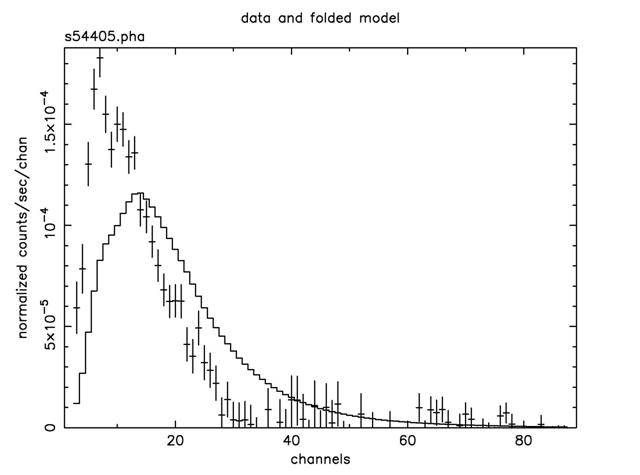
Figure B: The result of the command plot data after the command ignore bad on the EXOSAT ME spectrum 1E1048.1–5937
We can see that 40 channels are bad—but do we need to ignore any more? These channels are bad because of certain instrument properties: other channels still may need to be ignored because of the shape and brightness of the spectrum itself. Figure B shows the result of plotting the data in channels (using the commands setplot channel and plot data). We see that above about channel 33 the S/N becomes small. We also see, comparing Figure B with Figure A, which bad channels were ignored. Although visual inspection is not the most rigorous method for deciding which channels to ignore (more on this subject later), it's good enough for now, and will at least prevent us from getting grossly misleading results from the fitting. To ignore channels above 33:
XSPEC12> ignore 34-**
Chi-Squared = 677.6218 using 31 PHA bins.
Reduced chi-squared = 24.20078 for 28 degrees of freedom
Null hypothesis probability = 0.
The same result can be achieved with the command ignore 34–125. The inverse of ignore is notice, which has the same syntax.
We are now ready to fit the data. Fitting is initiated by
the command fit. As the fit proceeds, the screen displays the status of
the fit for each iteration until either the fit converges to the minimum ![]() , or the user
is asked whether the fit is to go through another set of iterations to find the
minimum. The default number of iterations is ten.
, or the user
is asked whether the fit is to go through another set of iterations to find the
minimum. The default number of iterations is ten.
XSPEC12>fit
Chi-Squared Lvl Fit param # 1 2 3
204.136 -3 7.9869E-02 1.564 4.4539E-03
84.5658 -4 0.3331 2.234 1.0977E-02
30.2511 -5 0.4422 2.174 1.1965E-02
30.1202 -6 0.4648 2.196 1.2264E-02
30.1189 -7 0.4624 2.195 1.2244E-02
---------------------------------------------------------------------------
Variances and Principal axes :
1 2 3
4.14E-08 | 0.00 -0.01 1.00
8.70E-02 | -0.91 -0.41 -0.01
2.32E-03 | -0.41 0.91 0.01
---------------------------------------------------------------------------
---------------------------------------------------------------------------
Model: phabs[1]( powerlaw[2] )
Model Fit Model Component Parameter Unit Value
par par comp
1 1 1 phabs nH 10^22 0.4624 +/- 0.2698
2 2 2 powerlaw PhoIndex 2.195 +/- 0.1288
3 3 2 powerlaw norm 1.2244E-02 +/- 0.2415E-02
---------------------------------------------------------------------------
---------------------------------------------------------------------------
Chi-Squared = 30.11890 using 31 PHA bins.
Reduced chi-squared = 1.075675 for 28 degrees of freedom
Null hypothesis probability = 0.358
The fit is good: reduced ![]() is 1.075 for 31 – 3 = 28 degrees of freedom. The null
hypothesis probability is the probability of getting a value of
is 1.075 for 31 – 3 = 28 degrees of freedom. The null
hypothesis probability is the probability of getting a value of ![]() as large or
larger than observed if the model is correct. If this probability is small then
the model is not a good fit. The matrix of principal axes printed out at the
end of a fit provides an indication of whether parameters are correlated (at
least local to the best fit). In this example the powerlaw norm is not
correlated with any other parameter while the column and powerlaw index are
slightly correlated. To see the fit and the residuals, we use the command
as large or
larger than observed if the model is correct. If this probability is small then
the model is not a good fit. The matrix of principal axes printed out at the
end of a fit provides an indication of whether parameters are correlated (at
least local to the best fit). In this example the powerlaw norm is not
correlated with any other parameter while the column and powerlaw index are
slightly correlated. To see the fit and the residuals, we use the command
XSPEC12>plot data resid
The result is shown in Figure C.
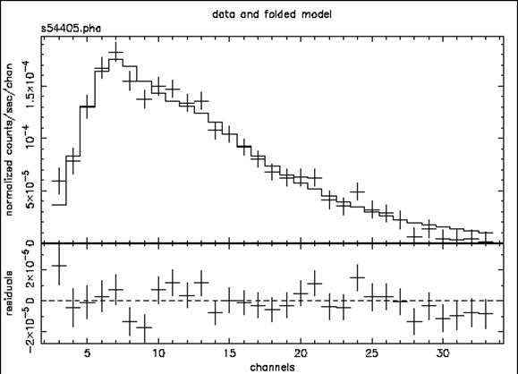
Figure C: The result of the command plot data with: the ME data file from 1E1048.1—5937; “bad” and negative channels ignored; the best-fitting absorbed power-law model; the residuals of the fit.
The screen output shows the best-fitting parameter values, as well as approximations to their errors. These errors should be regarded as indications of the uncertainties in the parameters and should not be quoted in publications. The true errors, i.e. the confidence ranges, are obtained using the error command:
XSPEC12>error 1 2 3
Parameter Confidence Range ( 2.706)
1 3.254765E-02 0.932778
2 1.99397 2.40950
*WARNING*:RENORM: No variable model to allow renormalization
*WARNING*:RENORM: No variable model to allow renormalization
*WARNING*:RENORM: No variable model to allow renormalization
*WARNING*:RENORM: No variable model to allow renormalization
*WARNING*:RENORM: No variable model to allow renormalization
*WARNING*:RENORM: No variable model to allow renormalization
*WARNING*:RENORM: No variable model to allow renormalization
*WARNING*:RENORM: No variable model to allow renormalization
*WARNING*:RENORM: No variable model to allow renormalization
*WARNING*:RENORM: No variable model to allow renormalization
8.942987E-03 1.711637E-02
Here, the numbers 1, 2, 3 refer to the parameter numbers in
the Model par
column of the screen output. For the first parameter, the column of absorbing
hydrogen atoms, the 90% confidence range is ![]() . This corresponds to an excursion
in
. This corresponds to an excursion
in ![]() of 2.706. The
reason these “better” errors are not given automatically as part of the fit
output is that they entail further fitting. When the model is simple, this does
not require much CPU, but for complicated models the extra time can be
considerable. The warning message is generated because there are no free
normalizations in the model while the error is being calculated on the
normalization itself. In this case, the warning may safely be ignored.
of 2.706. The
reason these “better” errors are not given automatically as part of the fit
output is that they entail further fitting. When the model is simple, this does
not require much CPU, but for complicated models the extra time can be
considerable. The warning message is generated because there are no free
normalizations in the model while the error is being calculated on the
normalization itself. In this case, the warning may safely be ignored.
What else can we do with the fit? One thing is to derive the flux of the model. The data by themselves only give the instrument-dependent count rate. The model, on the other hand, is an estimate of the true spectrum emitted. In XSPEC, the model is defined in physical units independent of the instrument. The command flux integrates the current model over the range specified by the user:
XSPEC12> flux 2 10
Model flux 3.5496E-03 photons ( 2.2492E-11 ergs)cm**-2 s**-1 ( 2.000- 10.000)
Here we have chosen the standard X-ray range of 2—10 keV and
find that the energy flux is ![]() Note that flux will integrate
only within the energy range of the current response matrix. If the model flux
outside this range is desired—in effect, an extrapolation beyond the
data---then the command dummyrsp should be used. This command sets up a
dummy response that covers the range required. For example, if we want to know
the flux of our model in the ROSAT PSPC band of 0.2—2 keV, we enter:
Note that flux will integrate
only within the energy range of the current response matrix. If the model flux
outside this range is desired—in effect, an extrapolation beyond the
data---then the command dummyrsp should be used. This command sets up a
dummy response that covers the range required. For example, if we want to know
the flux of our model in the ROSAT PSPC band of 0.2—2 keV, we enter:
XSPEC12>dummy 0.2 2.
Chi-Squared = 3583.779 using 31 PHA bins.
Reduced chi-squared = 127.9921 for 28 degrees of freedom
Null hypothesis probability = 0.
XSPEC12>flux 0.2 2.
Model flux 4.5306E-03 photons ( 9.1030E-12 ergs)cm**-2 s**-1 ( 0.200- 2.000)
The energy flux, at ![]() is lower in this band but the photon
flux is higher. To get our original response matrix back we enter:
is lower in this band but the photon
flux is higher. To get our original response matrix back we enter:
XSPEC12> response
Chi-Squared = 30.11890 using 31 PHA bins.
Reduced chi-squared = 1.075675 for 28 degrees of freedom
Null hypothesis probability = 0.358
The fit, as we've remarked, is good, and the parameters are constrained. But unless the purpose of our investigation is merely to measure a photon index, it's a good idea to check whether alternative models can fit the data just as well. We also should derive upper limits to components such as iron emission lines and additional continua, which, although not evident in the data nor required for a good fit, are nevertheless important to constrain. First, let's try an absorbed black body:
XSPEC12>mo pha(bb)
Model: phabs[1]( bbody[2] )
Input parameter value, delta, min, bot, top, and max values for ...
Current: 1 0.001 0 0 1E+05 1E+06
phabs:nH>/*
---------------------------------------------------------------------------
---------------------------------------------------------------------------
Model: phabs[1]( bbody[2] )
Model Fit Model Component Parameter Unit Value
par par comp
1 1 1 phabs nH 10^22 1.000 +/- 0.
2 2 2 bbody kT keV 3.000 +/- 0.
3 3 2 bbody norm 1.000 +/- 0.
---------------------------------------------------------------------------
---------------------------------------------------------------------------
Chi-Squared = 3.3142067E+09 using 31 PHA bins.
Reduced chi-squared = 1.1836453E+08 for 28 degrees of freedom
Null hypothesis probability = 0.
XSPEC12>fit
Chi-Squared Lvl Fit param # 1 2 3
1420.96 0 0.2116 2.987 7.7666E-04
1387.72 0 4.4419E-02 2.975 7.7003E-04
1376.39 0 4.3009E-03 2.963 7.6354E-04
1371.67 0 1.8192E-03 2.951 7.5730E-04
1367.04 0 5.8100E-04 2.939 7.5130E-04
1362.47 0 1.9059E-04 2.926 7.4548E-04
1357.84 0 6.1455E-05 2.913 7.3982E-04
1353.14 0 2.5356E-05 2.900 7.3429E-04
1348.36 0 6.7582E-06 2.887 7.2885E-04
1343.50 0 2.0479E-06 2.874 7.2350E-04
Number of trials exceeded - last iteration delta = 4.861
Continue fitting? (Y)y
...
113.954 0 0. 0.8907 2.7865E-04
113.954 -1 0. 0.8905 2.7859E-04
113.954 4 0. 0.8905 2.7859E-04
---------------------------------------------------------------------------
Variances and Principal axes :
2 3
2.88E-04 | -1.00 0.00
8.45E-11 | 0.00 -1.00
---------------------------------------------------------------------------
---------------------------------------------------------------------------
Model: phabs[1]( bbody[2] )
Model Fit Model Component Parameter Unit Value
par par comp
1 1 1 phabs nH 10^22 0. +/- -1.000
2 2 2 bbody kT keV 0.8905 +/- 0.1696E-01
3 3 2 bbody norm 2.7859E-04 +/- 0.9268E-05
---------------------------------------------------------------------------
---------------------------------------------------------------------------
Chi-Squared = 113.9542 using 31 PHA bins.
Reduced chi-squared = 4.069792 for 28 degrees of freedom
Null hypothesis probability = 2.481E-12
Note that when more than 10 iterations are required for convergence the user is asked whether or not to continue at the end of each set of 10. Saying no at these prompts is a good idea if the fit is not converging quickly. Conversely, to avoid having to keep answering the question, i.e., to increase the number of iterations before the prompting question appears, begin the fit with, say fit 100. This command will put the fit through 100 iterations before pausing.
Plotting the data and residuals again with
XSPEC12> plot data resid
we obtain Figure D:
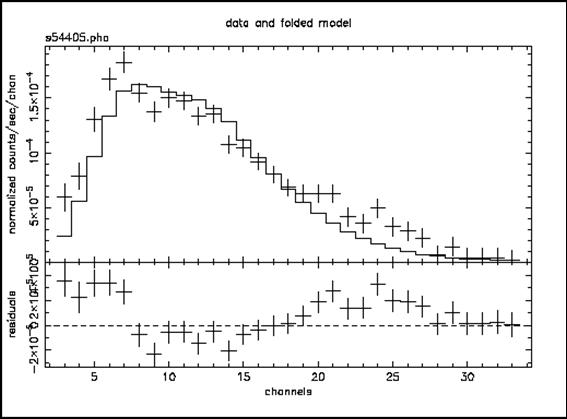
Figure D: As for Figure C, but the model is the best-fitting absorbed black body. Note the wave-like shape of the residuals which indicates how poor the fit is, i.e. that the continuum is obviously not a black body.
The black body fit is obviously not a good one. Not only is ![]() large, but the
best-fitting NH is rather low. Inspection of the residuals
confirms this: the pronounced wave-like shape is indicative of a bad choice of
overall continuum (see Figure D). Let's try thermal bremsstrahlung next:
large, but the
best-fitting NH is rather low. Inspection of the residuals
confirms this: the pronounced wave-like shape is indicative of a bad choice of
overall continuum (see Figure D). Let's try thermal bremsstrahlung next:
XSPEC12>mo pha(br)
Model: phabs[1]( bremss[2] )
Input parameter value, delta, min, bot, top, and max values for ...
Current: 1 0.001 0 0 1E+05 1E+06
phabs:nH>/*
---------------------------------------------------------------------------
---------------------------------------------------------------------------
Model: phabs[1]( bremss[2] )
Model Fit Model Component Parameter Unit Value
par par comp
1 1 1 phabs nH 10^22 1.000 +/- 0.
2 2 2 bremss kT keV 7.000 +/- 0.
3 3 2 bremss norm 1.000 +/- 0.
---------------------------------------------------------------------------
---------------------------------------------------------------------------
Chi-Squared = 4.5311800E+07 using 31 PHA bins.
Reduced chi-squared = 1618279. for 28 degrees of freedom
Null hypothesis probability = 0.
XSPEC12>fit
Chi-Squared Lvl Fit param # 1 2 3
113.305 -3 0.2441 6.557 6.8962E-03
40.4519 -4 0.1173 5.816 7.7944E-03
36.0549 -5 4.4750E-02 5.880 7.7201E-03
33.4168 -6 1.8882E-02 5.868 7.7476E-03
32.6766 -7 7.8376E-03 5.864 7.7495E-03
32.3192 -8 2.7059E-03 5.862 7.7515E-03
32.1512 -9 2.3222E-04 5.861 7.7525E-03
32.1471 -10 1.0881E-04 5.861 7.7523E-03
---------------------------------------------------------------------------
Variances and Principal axes :
1 2 3
2.29E-08 | 0.00 0.00 1.00
3.18E-02 | 0.95 0.31 0.00
8.25E-01 | 0.31 -0.95 0.00
---------------------------------------------------------------------------
---------------------------------------------------------------------------
Model: phabs[1]( bremss[2] )
Model Fit Model Component Parameter Unit Value
par par comp
1 1 1 phabs nH 10^22 1.0881E-04 +/- 0.3290
2 2 2 bremss kT keV 5.861 +/- 0.8651
3 3 2 bremss norm 7.7523E-03 +/- 0.8122E-03
---------------------------------------------------------------------------
---------------------------------------------------------------------------
Chi-Squared = 32.14705 using 31 PHA bins.
Reduced chi-squared = 1.148109 for 28 degrees of freedom
Null hypothesis probability = 0.269
Bremsstrahlung is a better fit than the black body—and is as good as the power law—although it shares the low NH. With two good fits, the power law and the bremsstrahlung, it's time to scrutinize their parameters in more detail.
First, we reset our fit to the powerlaw (output omitted):
XSPEC12>mo pha(po)
From the EXOSAT database on HEASARC, we know that the
target in question, 1E1048.1--5937, has a Galactic latitude of ![]() , i.e., almost on
the plane of the Galaxy. In fact, the database also provides the value of the
Galactic NH based on 21-cm radio observations. At
, i.e., almost on
the plane of the Galaxy. In fact, the database also provides the value of the
Galactic NH based on 21-cm radio observations. At ![]() , it is
higher than the 90 percent-confidence upper limit from the power-law fit.
Perhaps, then, the power-law fit is not so good after all. What we can do is
fix (freeze in XSPEC terminology) the value of NH at
the Galactic value and refit the power law. Although we won't get a good fit,
the shape of the residuals might give us a clue to what is missing. To freeze a
parameter in XSPEC, use the command freeze followed by the parameter
number, like this:
, it is
higher than the 90 percent-confidence upper limit from the power-law fit.
Perhaps, then, the power-law fit is not so good after all. What we can do is
fix (freeze in XSPEC terminology) the value of NH at
the Galactic value and refit the power law. Although we won't get a good fit,
the shape of the residuals might give us a clue to what is missing. To freeze a
parameter in XSPEC, use the command freeze followed by the parameter
number, like this:
XSPEC12> freeze 1
Number of variable fit parameters = 2
The inverse of freeze is thaw:
XSPEC12> thaw 1
Number of variable fit parameters = 3
Alternatively, parameters can be frozen using the newpar
command, which allows all the quantities associated with a parameter to be
changed. The second quantity, delta,
is the step size used to calculate the derivative in the fitting, and, if set
to a negative number, will cause the parameter to be frozen. In our case, we
want NH frozen at ![]() ,
so we go back to the power law best fit and do the following :
,
so we go back to the power law best fit and do the following :
XSPEC12>newpar 1
Current: 0.463 0.001 0 0 1E+05 1E+06
phabs:nH>4,0
---------------------------------------------------------------------------
---------------------------------------------------------------------------
Model: phabs[1]( powerlaw[2] )
Model Fit Model Component Parameter Unit Value
par par comp
1 1 1 phabs nH 10^22 4.000 frozen
2 2 2 powerlaw PhoIndex 2.195 +/- 0.1287
3 3 2 powerlaw norm 1.2247E-02 +/- 0.2412E-02
---------------------------------------------------------------------------
---------------------------------------------------------------------------
2 variable fit parameters
Chi-Squared = 829.3545 using 31 PHA bins.
Reduced chi-squared = 28.59843 for 29 degrees of freedom
Null hypothesis probability = 0.
Note the useful trick of giving a value of zero for delta in the newpar command. This has the effect of changing delta to the negative of its current value. If the parameter is free, it will be frozen, and if frozen, thawed. The same result can be obtained by putting everything onto the command line, i.e., newpar 1 4, 0, or by issuing the two commands, newpar 1 4 followed by freeze 1. Now, if we fit and plot again, we get the following model (Fig. E).
XSPEC12>fit
...
---------------------------------------------------------------------------
---------------------------------------------------------------------------
Model: phabs[1]( powerlaw[2] )
Model Fit Model Component Parameter Unit Value
par par comp
1 1 1 phabs nH 10^22 4.000 frozen
2 2 2 powerlaw PhoIndex 3.594 +/- 0.6867E-01
3 3 2 powerlaw norm 0.1161 +/- 0.9412E-02
---------------------------------------------------------------------------
---------------------------------------------------------------------------
Chi-Squared = 125.5134 using 31 PHA bins.
Reduced chi-squared = 4.328048 for 29 degrees of freedom
Null hypothesis probability = 5.662E-14
XSPEC12>plot data resid
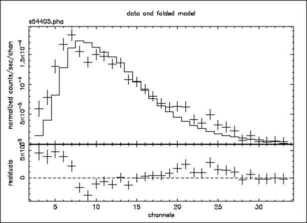
Figure E: As for Figure C & D, but the model is the best-fitting power law with the absorption fixed at the Galactic value. Under the assumptions that the absorption really is the same as the 21-cm value and that the continuum really is a power law, this plot provides some indication of what other components might be added to the model to improve the fit.
The fit is not good. In Figure E we can see why: there appears to be a surplus of softer photons, perhaps indicating a second continuum component. To investigate this possibility we can add a component to our model. The editmod command lets us do this without having to respecify the model from scratch. Here, we'll add a black body component.
XSPEC12>editmod pha(po+bb)
Model: phabs[1]( powerlaw[2] + bbody[3] )
Input parameter value, delta, min, bot, top, and max values for ...
Current: 3 0.01 0.0001 0.01 100 200
bbody:kT>2,0
Current: 1 0.01 0 0 1E+24 1E+24
bbody:norm>1.e-5
---------------------------------------------------------------------------
---------------------------------------------------------------------------
Model: phabs[1]( powerlaw[2] + bbody[3] )
Model Fit Model Component Parameter Unit Value
par par comp
1 1 1 phabs nH 10^22 4.000 frozen
2 2 2 powerlaw PhoIndex 3.594 +/- 0.6867E-01
3 3 2 powerlaw norm 0.1161 +/- 0.9412E-02
4 4 3 bbody kT keV 2.000 frozen
5 5 3 bbody norm 1.0000E-05 +/- 0.
---------------------------------------------------------------------------
---------------------------------------------------------------------------
Chi-Squared = 122.1538 using 31 PHA bins.
Reduced chi-squared = 4.362635 for 28 degrees of freedom
Null hypothesis probability = 9.963E-14
Notice that in specifying the initial values of the black body, we have frozen kT at 2 keV (the canonical temperature for nuclear burning on the surface of a neutron star in a low-mass X-ray binary) and started the normalization at zero. Without these measures, the fit might “lose its way”. Now, if we fit, we get (not showing all the iterations this time):
---------------------------------------------------------------------------
Model: phabs[1]( powerlaw[2] + bbody[3] )
Model Fit Model Component Parameter Unit Value
par par comp
1 1 1 phabs nH 10^22 4.000 frozen
2 2 2 powerlaw PhoIndex 4.932 +/- 0.1618
3 3 2 powerlaw norm 0.3761 +/- 0.5449E-01
4 4 3 bbody kT keV 2.000 frozen
5 5 3 bbody norm 2.3212E-04 +/- 0.3966E-04
---------------------------------------------------------------------------
---------------------------------------------------------------------------
Chi-Squared = 55.63374 using 31 PHA bins.
Reduced chi-squared = 1.986919 for 28 degrees of freedom
Null hypothesis probability = 1.425E-03
The fit is better than the one with just a power law and the fixed Galactic column, but it is still not good. Thawing the black body temperature and fitting gives us:
XSPEC12>thaw 4
Number of variable fit parameters = 4
XSPEC12>fit
...
---------------------------------------------------------------------------
---------------------------------------------------------------------------
Model: phabs[1]( powerlaw[2] + bbody[3] )
Model Fit Model Component Parameter Unit Value
par par comp
1 1 1 phabs nH 10^22 4.000 frozen
2 2 2 powerlaw PhoIndex 6.401 +/- 0.3873
3 3 2 powerlaw norm 1.086 +/- 0.3032
4 4 3 bbody kT keV 1.199 +/- 0.8082E-01
5 5 3 bbody norm 2.6530E-04 +/- 0.3371E-04
---------------------------------------------------------------------------
---------------------------------------------------------------------------
Chi-Squared = 37.21207 using 31 PHA bins.
Reduced chi-squared = 1.378225 for 27 degrees of freedom
Null hypothesis probability = 9.118E-02
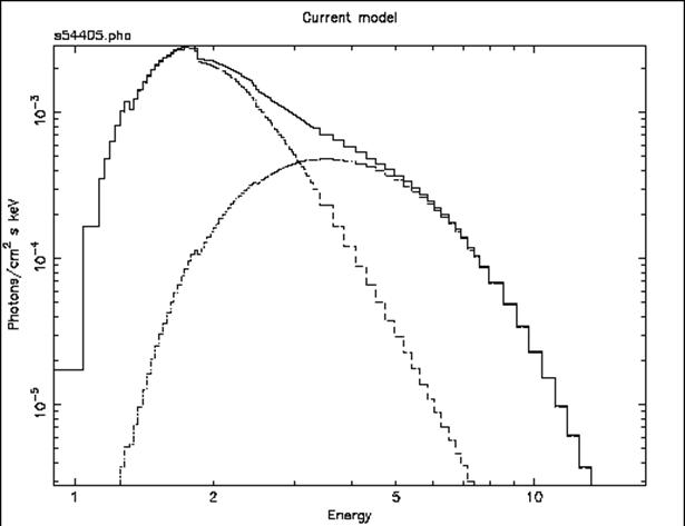
Figure F: The result of the command plot model in the case of the ME data file from 1E1048.1—5937. Here, the model is the best-fitting combination of power law, black body and fixed Galactic absorption. The three lines show the two continuum components (absorbed to the same degree) and their sum.
This, of course, is a better fit, but the photon index of the power law has ended up extremely and implausibly steep. Looking at this odd model with the command
XSPEC12> plot model
we see, in Figure F, that the black body and the power law have changed places, in that the power law provides the soft photons required by the high absorption, while the black body provides the harder photons.
We could continue to search for a plausible, well-fitting model, but the data, with their limited signal-to-noise and energy resolution, probably don't warrant it (the original investigators published only the power law fit). There is, however, one final, useful thing to do with the data: derive an upper limit to the presence of a fluorescent iron emission line. First we delete the black body component using delcomp:
XSPEC12>delcomp 3
Model: phabs[1]( powerlaw[2] )
Chi-Squared = 1285.487 using 31 PHA bins.
Reduced chi-squared = 44.32712 for 29 degrees of freedom
Then we thaw NH and refit to recover our original, best fit:
XSPEC12>thaw 1
Number of variable fit parameters = 3
XSPEC12>fit
Chi-Squared Lvl Fit param # 1 2 3
924.178 -2 5.087 5.076 0.4056
305.507 -2 4.525 3.791 0.1249
140.460 -2 2.930 3.367 6.5553E-02
64.4275 -3 0.6068 2.244 1.4635E-02
30.3738 -4 0.4837 2.201 1.2279E-02
30.1189 -5 0.4641 2.195 1.2258E-02
30.1189 -6 0.4637 2.195 1.2255E-02
---------------------------------------------------------------------------
Variances and Principal axes :
1 2 3
4.13E-08 | 0.00 -0.01 1.00
8.69E-02 | -0.91 -0.41 -0.01
2.31E-03 | -0.41 0.91 0.01
---------------------------------------------------------------------------
---------------------------------------------------------------------------
Model: phabs[1]( powerlaw[2] )
Model Fit Model Component Parameter Unit Value
par par comp
1 1 1 phabs nH 10^22 0.4637 +/- 0.2696
2 2 2 powerlaw PhoIndex 2.195 +/- 0.1287
3 3 2 powerlaw norm 1.2255E-02 +/- 0.2412E-02
---------------------------------------------------------------------------
---------------------------------------------------------------------------
Chi-Squared = 30.11890 using 31 PHA bins.
Reduced chi-squared = 1.075675 for 28 degrees of freedom
Null hypothesis probability = 0.358
Now, we add a gaussian emission line of fixed energy and width:
XSPEC12>editmod pha(po+ga)
Model: phabs[1]( powerlaw[2] + gaussian[3] )
Input parameter value, delta, min, bot, top, and max values for ...
Current: 6.5 0.05 0 0 1E+06 1E+06
gaussian:LineE>6.4 0
Current: 0.1 0.05 0 0 10 20
gaussian:Sigma>0.1 0
Current: 1 0.01 0 0 1E+24 1E+24
gaussian:norm>1.e-4
---------------------------------------------------------------------------
---------------------------------------------------------------------------
Model: phabs[1]( powerlaw[2] + gaussian[3] )
Model Fit Model Component Parameter Unit Value
par par comp
1 1 1 phabs nH 10^22 0.4637 +/- 0.2696
2 2 2 powerlaw PhoIndex 2.195 +/- 0.1287
3 3 2 powerlaw norm 1.2255E-02 +/- 0.2412E-02
4 4 3 gaussian LineE keV 6.400 frozen
5 5 3 gaussian Sigma keV 0.1000 frozen
6 6 3 gaussian norm 1.0000E-04 +/- 0.
---------------------------------------------------------------------------
---------------------------------------------------------------------------
Chi-Squared = 32.75002 using 31 PHA bins.
Reduced chi-squared = 1.212964 for 27 degrees of freedom
Null hypothesis probability = 0.205
XSPEC12>fit
...
---------------------------------------------------------------------------
---------------------------------------------------------------------------
Model: phabs[1]( powerlaw[2] + gaussian[3] )
Model Fit Model Component Parameter Unit Value
par par comp
1 1 1 phabs nH 10^22 0.6562 +/- 0.3193
2 2 2 powerlaw PhoIndex 2.324 +/- 0.1700
3 3 2 powerlaw norm 1.4636E-02 +/- 0.3642E-02
4 4 3 gaussian LineE keV 6.400 frozen
5 5 3 gaussian Sigma keV 0.1000 frozen
6 6 3 gaussian norm 9.6462E-05 +/- 0.9542E-04
---------------------------------------------------------------------------
---------------------------------------------------------------------------
Chi-Squared = 29.18509 using 31 PHA bins.
Reduced chi-squared = 1.080929 for 27 degrees of freedom
Null hypothesis probability = 0.352
The energy and width have to be frozen because, in the absence of an obvious line in the data, the fit would be completely unable to converge on meaningful values. Besides, our aim is to see how bright a line at 6.4 keV can be and still not ruin the fit. To do this, we fit first and then use the error command to derive the maximum allowable iron line normalization. We then set the normalization at this maximum value with newpar and, finally, derive the equivalent width using the eqwidth command. That is:
XSPEC12>err 6
Parameter Confidence Range ( 2.706)
Parameter pegged at hard limit 0.
with delta ftstat= 0.9338
6 0. 1.530722E-04
XSPEC12>new 6 1.530722E-04
4 variable fit parameters
Chi-Squared = 34.91923 using 31 PHA bins.
Reduced chi-squared = 1.293305 for 27 degrees of freedom
Null hypothesis probability = 0.141
XSPEC12>eqwidth 3
Additive group equiv width for model 3 (gaussian): 839. eV
Things to note:
The true minimum value of the gaussian normalization is less
than zero, but the error command stopped searching for a ![]() of 2.706
when the minimum value hit zero, the “hard” lower limit of the parameter. Hard
limits can be adjusted with the newpar command, and they correspond to
the quantities min
and max
associated with the parameter values. In fact, according to the screen output,
the value of
of 2.706
when the minimum value hit zero, the “hard” lower limit of the parameter. Hard
limits can be adjusted with the newpar command, and they correspond to
the quantities min
and max
associated with the parameter values. In fact, according to the screen output,
the value of ![]() corresponding
to zero normalization is 0.934.
corresponding
to zero normalization is 0.934.
The command eqwidth takes the component number as its argument.
The upper limit on the equivalent width of a 6.4 keV emission line is high (839 eV)!
Simultaneous Fitting: Examples from Einstein and Ginga
XSPEC has the very useful facility of allowing models to be fitted simultaneously to more than one data file. It is even possible to group files together and to fit different models simultaneously. Reasons for fitting in this manner include:
The same target is observed at several epochs but, although the source stays constant, the response matrix has changed. When this happens, the data files cannot be added together; they have to be fitted separately. Fitting the data files simultaneously yields tighter constraints.
The same target is observed with different instruments. The GIS and SIS on ASCA, for example, observe in the same direction simultaneously. As far as XSPEC is concerned, this is just like the previous case: two data files with two responses fitted simultaneously with the same model.
Different targets are observed, but the user wants to fit the same model to each data file with some parameters shared and some allowed to vary separately. For example, if you have a series of spectra from a variable AGN, you might want to fit them simultaneously with a model that has the same, common photon index but separately vary the normalization and absorption.
Other scenarios are possible---the important thing is to recognize the flexibility of XSPEC in this regard.
As an example of the first case, we'll fit two spectra derived from two separate Einstein Solid State Spectrometer (SSS) observations of the cooling-flow cluster Abell 496. Although the two observations were carried out on consecutive days (in August 1979), the response is different, due to the variable build-up of ice on the detector. This problem bedeviled analysis during the mission; however, it has now been calibrated successfully and is incorporated into the response matrices associated with the spectral files in the HEASARC archive. The SSS also provides an example of how background correction files are used in XSPEC.
To fit the same model with the same set of parameters to more than one data file, simply enter the names of the data files after the data command:
XSPEC12> data sa496b.pha sa496c.pha
Net count rate (cts/s) for file 1 0.7806 +/- 9.3808E+05( 86.9% total)
using response (RMF) file... sa496b.rsp
using background file... sa496b.bck
using correction file... sa496b.cor
Net count rate (cts/s) for file 2 0.8002 +/- 9.3808E+05( 86.7% total)
using response (RMF) file... sa496c.rsp
using background file... sa496c.bck
using correction file... sa496c.cor
Net correction flux for file 1= 8.4469E-04
Net correction flux for file 2= 8.7577E-04
2 data sets are in use
As the messages indicate, XSPEC also has read in the associated:
response files (sa496b.rsp & sa496c.rsp),
background files (sa496b.bck& sa496c.bck) and
correction files (sa496b.cor & sa496c.cor).
These files are all listed in the headers of the data files (sa496b.pha & sa496c.pha).
To ignore channels, the file number (1 & 2 in this example) precedes the range of channels to be ignored. Here, we wish to ignore, for both files, channels 1—15 and channels 100—128. This can be done by specifying the files one after the other with the range of ignored channels:
XSPEC12> ignore 1:1-15 1:100-128 2:1-15 2:100-128
Chi-Squared = 1933.559 using 168 PHA bins.
Reduced chi-squared = 11.79000 for 164 degrees of freedom
Null hypothesis probability = 0.
or by specifying the range of file number with the channel range:
XSPEC12> ignore 1-2:1-15 100-128
In this example, we'll fit a cooling-flow model under the reasonable assumption that the small SSS field of view sees mostly just the cool gas in the middle of the cluster. We'll freeze the values of the maximum temperature (the temperature from which the gas cools) and of the abundance to the values found by instruments such as the Ginga LAC and the EXOSAT ME, which observed the entire cluster. The minimum gas temperature is frozen at 0.1 keV; the “slope” is frozen at zero (isobaric cooling) and the normalization is given an initial value of 100 solar masses per year:
XSPEC12>mo pha(cflow)
Model: phabs[1]( cflow[2] )
Input parameter value, delta, min, bot, top, and max values for ...
Current: 1 0.001 0 0 1E+05 1E+06
phabs:nH>0.045
Current: 0 0.01 -5 -5 5 5
cflow:slope>0,0
Current: 0.1 0.001 0.0808 0.0808 79.9 79.9
cflow:lowT>0.1,0
Current: 4 0.001 0.0808 0.0808 79.9 79.9
cflow:highT>4,0
Current: 1 0.01 0 0 5 5
cflow:Abundanc>0.5,0
Current: 0 -0.1 0 0 100 100
cflow:Redshift>0.032
Current: 1 0.01 0 0 1E+24 1E+24
cflow:norm>100
---------------------------------------------------------------------------
---------------------------------------------------------------------------
Model: phabs[1]( cflow[2] )
Model Fit Model Component Parameter Unit Value
par par comp
1 1 1 phabs nH 10^22 4.5000E-02 +/- 0.
2 2 2 cflow slope 0. frozen
3 3 2 cflow lowT keV 0.1000 frozen
4 4 2 cflow highT keV 4.000 frozen
5 5 2 cflow Abundanc 0.5000 frozen
6 6 2 cflow Redshift 3.2000E-02 frozen
7 7 2 cflow norm 100.0 +/- 0.
---------------------------------------------------------------------------
---------------------------------------------------------------------------
Chi-Squared = 2740.606 using 168 PHA bins.
Reduced chi-squared = 16.50968 for 166 degrees of freedom
Null hypothesis probability = 0.
XSPEC12>fit
Chi-Squared Lvl Fit param # 1 2 3 4
5 6 7
414.248 -3 0.2050 0. 0.1000 4.000
0.5000 3.2000E-02 288.5
373.205 -4 0.2508 0. 0.1000 4.000
0.5000 3.2000E-02 321.9
372.649 -5 0.2566 0. 0.1000 4.000
0.5000 3.2000E-02 325.9
372.640 -6 0.2574 0. 0.1000 4.000
0.5000 3.2000E-02 326.3
---------------------------------------------------------------------------
Variances and Principal axes :
1 7
3.55E-05 | -1.00 0.00
3.52E+01 | 0.00 -1.00
---------------------------------------------------------------------------
---------------------------------------------------------------------------
Model: phabs[1]( cflow[2] )
Model Fit Model Component Parameter Unit Value
par par comp
1 1 1 phabs nH 10^22 0.2574 +/- 0.9219E-02
2 2 2 cflow slope 0. frozen
3 3 2 cflow lowT keV 0.1000 frozen
4 4 2 cflow highT keV 4.000 frozen
5 5 2 cflow Abundanc 0.5000 frozen
6 6 2 cflow Redshift 3.2000E-02 frozen
7 7 2 cflow norm 326.3 +/- 5.929
---------------------------------------------------------------------------
---------------------------------------------------------------------------
Chi-Squared = 372.6400 using 168 PHA bins.
Reduced chi-squared = 2.244819 for 166 degrees of freedom
Null hypothesis probability = 6.535E-18
As we can see, ![]() is
not good, but the high statistic could be because we have yet to adjust the
correction file. Correction files in XSPEC take into account detector features
that cannot be completely prescribed ab initio and which must be fitted
at the same time as the model. Einstein SSS spectra, for example, have a
background feature the level of which varies unpredictably. Its spectral form
is contained in the correction file, but its normalization is determined by
fitting. This fitting is set in motion using the command recornrm (
reset the correction-file normalization):
is
not good, but the high statistic could be because we have yet to adjust the
correction file. Correction files in XSPEC take into account detector features
that cannot be completely prescribed ab initio and which must be fitted
at the same time as the model. Einstein SSS spectra, for example, have a
background feature the level of which varies unpredictably. Its spectral form
is contained in the correction file, but its normalization is determined by
fitting. This fitting is set in motion using the command recornrm (
reset the correction-file normalization):
XSPEC12>reco 1
File # Correction
1 0.4118 +/- 0.0673
After correction norm adjustment 0.412 +/- 0.067
Chi-Squared = 335.1577 using 168 PHA bins.
Reduced chi-squared = 2.019022 for 166 degrees of freedom
Null hypothesis probability = 1.650E-13
XSPEC12>reco 2
File # Correction
2 0.4864 +/- 0.0597
After correction norm adjustment 0.486 +/- 0.060
Chi-Squared = 268.8205 using 168 PHA bins.
Reduced chi-squared = 1.619400 for 166 degrees of freedom
Null hypothesis probability = 7.552E-07
This process is iterative, and, in order to work must be
used in tandem with fitting the model. Successive fits and recorrections are
applied until the fit is stable, i.e., until further improvement in![]() no longer
results. Of course, this procedure is only worthwhile when the model gives a
reasonably good account of the data. Eventually, we end up at:
no longer
results. Of course, this procedure is only worthwhile when the model gives a
reasonably good account of the data. Eventually, we end up at:
XSPEC12>fit
Chi-Squared Lvl Fit param # 1 2 3 4
5 6 7
224.887 -3 0.2804 0. 0.1000 4.000
0.5000 3.2000E-02 313.0
224.792 -4 0.2835 0. 0.1000 4.000
0.5000 3.2000E-02 314.5
224.791 -5 0.2837 0. 0.1000 4.000
0.5000 3.2000E-02 314.6
---------------------------------------------------------------------------
Variances and Principal axes :
1 7
4.64E-05 | -1.00 0.00
3.78E+01 | 0.00 -1.00
---------------------------------------------------------------------------
---------------------------------------------------------------------------
Model: phabs[1]( cflow[2] )
Model Fit Model Component Parameter Unit Value
par par comp
1 1 1 phabs nH 10^22 0.2837 +/- 0.1051E-01
2 2 2 cflow slope 0. frozen
3 3 2 cflow lowT keV 0.1000 frozen
4 4 2 cflow highT keV 4.000 frozen
5 5 2 cflow Abundanc 0.5000 frozen
6 6 2 cflow Redshift 3.2000E-02 frozen
7 7 2 cflow norm 314.6 +/- 6.147
---------------------------------------------------------------------------
---------------------------------------------------------------------------
Chi-Squared = 224.7912 using 168 PHA bins.
Reduced chi-squared = 1.354164 for 166 degrees of freedom
Null hypothesis probability = 1.616E-03
The final value of ![]() is much better than the original, but is not quite
acceptable. However, the current model has only two free parameters: further
explorations of parameter space would undoubtedly improve the fit.
is much better than the original, but is not quite
acceptable. However, the current model has only two free parameters: further
explorations of parameter space would undoubtedly improve the fit.
We'll leave this example and move on to look at another kind of simultaneous fitting: one where the same model is fitted to two different data files. This time, not all the parameters will be identical. The massive X-ray binary Centaurus X-3 was observed with the LAC on Ginga in 1989. Its flux level before eclipse was much lower than the level after eclipse. Here, we'll use XSPEC to see whether spectra from these two phases can be fitted with the same model, which differs only in the amount of absorption. This kind of fitting relies on introducing an extra dimension, the group, to the indexing of the data files. The files in each group share the same model but not necessarily the same parameter values, which may be shared as common to all the groups or varied separately from group to group. Although each group may contain more than one file, there is only one file in each of the two groups in this example. Groups are specified with the data command, with the group number preceding the file number, like this:
XSPEC12> da 1:1 losum 2:2 hisum
Net count rate (cts/s) for file 1 140.1 +/- 0.3549
using response (RMF) file... ginga_lac.rsp
Net count rate (cts/s) for file 2 1371. +/- 3.123
using response (RMF) file... ginga_lac.rsp
2 data sets are in use
Here, the first group makes up the file losum.pha, which contains the spectrum of all the low, pre-eclipse emission. The second group makes up the second file, hisum.pha, which contains all the high, post-eclipse emission. Note that file number is “absolute” in the sense that it is independent of group number. Thus, if there were three files in each of the two groups (lo1.pha, lo2.pha, lo3.pha, hi1.pha, hi2.pha, and hi3.pha, say), rather than one, the six files would be specified as da 1:1 lo1 1:2 lo2 1:3 lo3 2:4 hi1 2:5 hi2 2:6 hi3. The ignore command works, as usual, on file number, and does not take group number into account. So, to ignore channels 1–3 and 37–48 of both files:
XSPEC12> ignore 1-2:1-3 37-48
The model we'll use at first to fit the two files is an absorbed power law with a high-energy cut-off:
XSPEC12> mo phabs * highecut (po)
After defining the model, the user is prompted for two sets of parameter values, one for the first group of data files (losum.pha), the other for the second group (hisum.pha). Here, we'll enter the absorption column of the first group as 1024 cm–2 and enter the default values for all the other parameters in the first group. Now, when it comes to the second group of parameters, we enter a column of 1022 cm–2 and then enter defaults for the other parameters. The rule being applied here is as follows: to tie parameters in the second group to their equivalents in the first group, take the default when entering the second-group parameters; to allow parameters in the second group to vary independently of their equivalents in the first group, enter different values explicitly:
XSPEC12>mo phabs*highecut(po)
Model: phabs[1]*highecut[2]( powerlaw[3] )
Input parameter value, delta, min, bot, top, and max values for ...
Current: 1 0.001 0 0 1E+05 1E+06
DataGroup 1:phabs:nH>100
Current: 10 0.01 0.0001 0.01 1E+06 1E+06
DataGroup 1:highecut:cutoffE>/
Current: 15 0.01 0.0001 0.01 1E+06 1E+06
DataGroup 1:highecut:foldE>/
Current: 1 0.01 -3 -2 9 10
DataGroup 1:powerlaw:PhoIndex>/
Current: 1 0.01 0 0 1E+24 1E+24
DataGroup 1:powerlaw:norm>/
Current: 100 0.001 0 0 1E+05 1E+06
DataGroup 2:phabs:nH>1
Current: 10 0.01 0.0001 0.01 1E+06 1E+06
DataGroup 2:highecut:cutoffE>/*
---------------------------------------------------------------------------
---------------------------------------------------------------------------
Model: phabs[1]*highecut[2]( powerlaw[3] )
Model Fit Model Component Parameter Unit Value Data
par par comp group
1 1 1 phabs nH 10^22 100.0 +/- 0. 1
2 2 2 highecut cutoffE keV 10.00 +/- 0. 1
3 3 2 highecut foldE keV 15.00 +/- 0. 1
4 4 3 powerlaw PhoIndex 1.000 +/- 0. 1
5 5 3 powerlaw norm 1.000 +/- 0. 1
6 6 4 phabs nH 10^22 1.000 +/- 0. 2
7 2 5 highecut cutoffE keV 10.00 = par 2 2
8 3 5 highecut foldE keV 15.00 = par 3 2
9 4 6 powerlaw PhoIndex 1.000 = par 4 2
10 5 6 powerlaw norm 1.000 = par 5 2
---------------------------------------------------------------------------
---------------------------------------------------------------------------
Chi-Squared = 2.0263934E+07 using 66 PHA bins.
Reduced chi-squared = 337732.2 for 60 degrees of freedom
Null hypothesis probability = 0.
Notice how the summary of the model, displayed immediately
above, is different now that we have two groups, as opposed to one (as in all
the previous examples). We can see that of the 10 model parameters, 6 are free
(i.e., 4 of the second group parameters are tied to their equivalents in the
first group). Fitting this model results in a huge ![]() (not shown here), because our assumption that only a
change in absorption can account for the spectral variation before and after
eclipse is clearly wrong. Perhaps scattering also plays a role in reducing the
flux before eclipse. This could be modeled (simply at first) by allowing the
normalization of the power law to be smaller before eclipse than after eclipse.
To decouple tied parameters, we change the parameter value in the second group
to a value—any value—different from that in the first group (changing the value
in the first group has the effect of changing both without decoupling). As
usual, the newpar command is used:
(not shown here), because our assumption that only a
change in absorption can account for the spectral variation before and after
eclipse is clearly wrong. Perhaps scattering also plays a role in reducing the
flux before eclipse. This could be modeled (simply at first) by allowing the
normalization of the power law to be smaller before eclipse than after eclipse.
To decouple tied parameters, we change the parameter value in the second group
to a value—any value—different from that in the first group (changing the value
in the first group has the effect of changing both without decoupling). As
usual, the newpar command is used:
XSPEC12>newpar 10 1
7 variable fit parameters
Chi-Squared = 2.0263934E+07 using 66 PHA bins.
Reduced chi-squared = 343456.5 for 59 degrees of freedom
Null hypothesis probability = 0.
XSPEC12>fit
...
---------------------------------------------------------------------------
Model: phabs[1]*highecut[2]( powerlaw[3] )
Model Fit Model Component Parameter Unit Value Data
par par comp group
1 1 1 phabs nH 10^22 20.23 +/- 0.1823 1
2 2 2 highecut cutoffE keV 14.68 +/- 0.5552E-01 1
3 3 2 highecut foldE keV 7.430 +/- 0.8945E-01 1
4 4 3 powerlaw PhoIndex 1.187 +/- 0.6505E-02 1
5 5 3 powerlaw norm 5.8958E-02 +/- 0.9334E-03 1
6 6 4 phabs nH 10^22 1.270 +/- 0.3762E-01 2
7 2 5 highecut cutoffE keV 14.68 = par 2 2
8 3 5 highecut foldE keV 7.430 = par 3 2
9 4 6 powerlaw PhoIndex 1.187 = par 4 2
10 7 6 powerlaw norm 0.3123 +/- 0.4513E-02 2
---------------------------------------------------------------------------
---------------------------------------------------------------------------
Chi-Squared = 15424.73 using 66 PHA bins.
Reduced chi-squared = 261.4362 for 59 degrees of freedom
Null hypothesis probability = 0.
After fitting, this decoupling reduces ![]() by a factor of
six to 15,478, but this is still too high. Indeed, this simple attempt to
account for the spectral variability in terms of “blanket” cold absorption and
scattering does not work. More sophisticated models, involving additional
components and partial absorption, should be investigated.
by a factor of
six to 15,478, but this is still too high. Indeed, this simple attempt to
account for the spectral variability in terms of “blanket” cold absorption and
scattering does not work. More sophisticated models, involving additional
components and partial absorption, should be investigated.
Using XSPEC to Simulate Data: an Example from ASCA
In several cases, analyzing simulated data is a powerful tool to demonstrate feasibility. For example:
To support an observing proposal. That is, to demonstrate what constraints a proposed observation would yield.
To support a hardware proposal. If a response matrix is generated, it can be used to demonstrate what kind of science could be done with a new instrument.
To support a theoretical paper. A theorist could write a paper describing a model, and then show how these model spectra would appear when observed. This, of course, is very like the first case.
Here, we'll use XSPEC to see how an ASCA observation of the elliptical galaxy NGC 4472 can constrain the condition of the hot gas. The first step is to define a model on which to base the simulation. The way XSPEC creates simulated data is to take the current model, convolve it with the current response matrix, while adding noise appropriate to the integration time specified. Once created, the simulated data can be analyzed in the same way as real data to derive confidence limits.
We begin by looking in the literature for the best estimate
of the NGC 4472 spectrum. BBXRT observed the galaxy in 1990 and the
results were published in Serlemitsos et al., (1993). They found a flux in the
0.5–4.5 keV range of ![]() , a temperature range of 0.74 < kT
< 0.98, an abundance range (as a fraction of solar) of 0.09 < A < 0.46
and a column range of
, a temperature range of 0.74 < kT
< 0.98, an abundance range (as a fraction of solar) of 0.09 < A < 0.46
and a column range of ![]() . A Raymond-Smith spectral
model was found to give a good fit. We specify this model at first with the
median parameter values, except for the normalization of the Raymond-Smith,
which we leave at its default value of unity at first (but adjust later):
. A Raymond-Smith spectral
model was found to give a good fit. We specify this model at first with the
median parameter values, except for the normalization of the Raymond-Smith,
which we leave at its default value of unity at first (but adjust later):
XSPEC12>mo pha(ray)
Model: phabs[1]( raymond[2] )
Input parameter value, delta, min, bot, top, and max values for ...
Current: 1 0.001 0 0 1E+05 1E+06
phabs:nH>0.21
Current: 1 0.01 0.008 0.008 64 64
raymond:kT>0.86
Current: 1 -0.001 0 0 5 5
raymond:Abundanc>0.27
Current: 0 -0.001 0 0 2 2
raymond:Redshift>/*
---------------------------------------------------------------------------
---------------------------------------------------------------------------
Model: phabs[1]( raymond[2] )
Model Fit Model Component Parameter Unit Value
par par comp
1 1 1 phabs nH 10^22 0.2100 +/- 0.
2 2 2 raymond kT keV 0.8600 +/- 0.
3 3 2 raymond Abundanc 0.2700 frozen
4 4 2 raymond Redshift 0. frozen
5 5 2 raymond norm 1.000 +/- 0.
---------------------------------------------------------------------------
---------------------------------------------------------------------------
We now can derive the correct normalization by using the commands dummyrsp, flux and newpar. That is, we'll determine the flux of the model with the normalization of unity (this requires a response matrix to cover the BBXRT band—we use a dummy response here). We then work out the new normalization and reset it:
XSPEC12> dummy 0.5 4.5
XSPEC12>flux 0.5 4.5
Model flux 0.2802 photons ( 4.9626E-10 ergs)cm**-2 s**-1 ( 0.500- 4.500)
XSPEC12> newpar 5 0.014
3 variable fit parameters
XSPEC12>flux
Model flux 3.9235E-03 photons ( 6.9476E-12 ergs)cm**-2 s**-1 ( 0.500- 4.500)
Here, we have changed the value of the normalization (the
fifth parameter) from 1 to ![]() to give the flux observed by BBXRT
(
to give the flux observed by BBXRT
(![]() in
the energy range 0.5–4.5).
in
the energy range 0.5–4.5).
The simulation is initiated with the command fakeit. If the argument none is given, the user will be prompted for the name of the response matrix. If no argument is given, the current response will be used:
XSPEC12>fakeit none
For fake data, file #1 needs response file: s0c1g0234p40e1_512_1av0_8i
... and ancillary response file: none
There then follows a series of prompts asking the user to specify whether he or she wants counting statistics (yes!), the name of the fake data (file ngc4472_sis.fak in our example), and the integration time T (40,000 seconds – cornorm can be left at its default value).
Use counting statistics in creating fake data? (y) /
Input optional fake file prefix (max 4 chars): /
Fake data filename (s0c1g0234p40e1_512_1av0_8i.fak) [/ to use default]: ngc4472_sis.fak
T, cornorm (1, 0): 40000
Net count rate (cts/s) for file 1 0.3563 +/- 3.0221E-03
using response (RMF) file... s0c1g0234p40e1_512_1av0_8i.rsp
Chi-Squared = 188.6545 using 512 PHA bins.
Reduced chi-squared = 0.3706375 for 509 degrees of freedom
Null hypothesis probability = 1.00
We now have created a file containing a simulated spectrum of NGC 4472. As is usual before fitting, we need to check which channels to ignore. This time, we'll examine the actual numbers of counts in each channel and reject those that have fewer than 20 per channel. We use iplot counts and see that our criterion requires us to ignore channels 1–15 and 76–512:
XSPEC12>ignore 1-15 76-**
Chi-Squared = 63.30437 using 60 PHA bins.
Reduced chi-squared = 1.110603 for 57 degrees of freedom
Null hypothesis probability = 0.264
As expected, ![]() is
reasonable even before fitting because the model and the data have the same
shape. But the point of this simulation is to determine confidence ranges.
First, we thaw the value of the abundance (fixed by default), fit and then use
the error command:
is
reasonable even before fitting because the model and the data have the same
shape. But the point of this simulation is to determine confidence ranges.
First, we thaw the value of the abundance (fixed by default), fit and then use
the error command:
XSPEC12> thaw 3
Number of variable fit parameters = 4
XSPEC12>fit
Chi-Squared Lvl Fit param # 1 2 3 4
5
55.3176 -3 0.2309 0.8569 0.2772 0.
1.4322E-02
55.2946 -4 0.2320 0.8565 0.2784 0.
1.4322E-02
55.2945 -5 0.2321 0.8565 0.2784 0.
1.4322E-02
-------------------------------------------------------------------------
Variances and Principal axes :
1 2 3 5
1.51E-08 | -0.03 -0.01 0.03 1.00
1.02E-05 | 0.39 0.91 -0.11 0.03
9.98E-05 | -0.91 0.40 0.11 -0.03
2.32E-04 | -0.15 -0.06 -0.99 0.03
-------------------------------------------------------------------------
-------------------------------------------------------------------------
Model: phabs[1]( raymond[2] )
Model Fit Model Component Parameter Unit Value
par par comp
1 1 1 phabs nH 10^22 0.2321 +/- 0.9426E-02
2 2 2 raymond kT keV 0.8565 +/- 0.5048E-02
3 3 2 raymond Abundanc 0.2784 +/- 0.1510E-01
4 4 2 raymond Redshift 0. frozen
5 5 2 raymond norm 1.4322E-02 +/- 0.5423E-03
-------------------------------------------------------------------------
-------------------------------------------------------------------------
Chi-Squared = 55.29454 using 60 PHA bins.
Reduced chi-squared = 0.9874024 for 56 degrees of freedom
Null hypothesis probability = 0.502
XSPEC12>err 1 2 3
Parameter Confidence Range ( 2.706)
1 0.217009 0.248102
2 0.847909 0.864666
3 0.254807 0.304992
These confidence ranges show that an ASCA observation would definitely constrain the parameters, especially the column and abundance, more tightly than the original BBXRT observation. Of course, whether these constraints are sufficient depends on the theories being tested. When producing and analyzing simulated data, it is crucial to keep in mind the purpose of the proposed observation, for the potential parameter space that can be covered with simulations is almost limitless.
Producing Plots: Modifying the Defaults
The final results of using XSPEC are usually one or more tables containing confidence ranges and fit statistics, and one or more plots showing the fits themselves. So far, all the plots shown have the default settings, but it is possible to edit plots to get closer to the appearance what you want.
The plotting package used by XSPEC is PGPLOT, which is comprised of a library of low-level tasks. At a higher level is QDP/PLT, the interactive program that forms the interface between the XSPEC user and PGPLOT. QDP/PLT has its own manual; it also comes with on-line help. Here, we show how to make some of the most common modifications to plots.
To initiate interactive plotting in XSPEC, use the command iplot instead of the usual plot. In this example, we'll take the simulated ASCA SIS spectrum of the previous section and make the following modifications to the data plot:
Change the aspect ratio
Change the labels
Rescale the x-axis and y-axis
Change the y-axis to be a logarithmic scale
Thicken the lines and make the characters smaller to make the hardcopy look better
Produce a postscript file
After the iplot command, the plot itself appears, followed by the QDP/PLT prompt:
XSPEC12> setplot energy
XSPEC12> iplot data
PLT>
The first thing we'll do is change the aspect ratio of the box that contains the plot (viewport in QDP terminology). The viewport is defined by the coordinates of the lower left and upper right corners of the page, normalized so that the width and height of the page are unity. The labels fall outside the viewport, so if the full viewport were specified, only the plot would appear. The default box has a viewport with corners at (0.1, 0.1) and (0.9, 0.9). For our purposes, we want a viewport with corners at (0.2, 0.2) and (0.8, 0.7): with this size and shape, the hardcopy will fit nicely on the page and not have to be reduced for photocopying. To change the viewport, use the command viewport followed by the coordinates:
PLT> viewport 0.2 0.2 0.8 0.7
Next we want to change two of the labels: the label at the top, which currently says only data, and the label that specifies the filename. This change is a straightforward one using the label command, which takes as arguments a location description and the text string:
PLT> label top Simulated Spectrum of NGC 4472
PLT> label file ASCA SIS
Other location descriptors are available, including x and y for the x-axis and y-axis, respectively. To get help on a QDP command, type help followed by the name of the command at the PLT> prompt. Note that QDP commands can be abbreviated, just like XSPEC commands. To see the results of changing the viewport and the labels, just enter the command plot:
PLT> plot
The two changes we want to make next are to rescale the axes and to change the y-axis to a logarithmic scale. The commands for these changes also are straightforward: the rescale command takes the minimum and maximum values as its arguments, while the log command takes x or y as arguments:
PLT> rescale x 0.4 2.5
PLT> rescale y 0.01 1
PLT> log y
PLT> plot
To revert to a linear scale, use the command log off y. All that is left to change are the thickness of the lines (the default, least for postscript files that are turned into hardcopies, is too fine) and the size of the characters (we want slightly smaller characters). The lwidth command does the former: it takes a width as its argument: the default is 1: we'll reset it to 3. The csize command does the latter, taking a normalization as its argument. One (1) will not change the size, a number less than one will reduce it and a number bigger than one will increase it.
PLT> lwidth 3
PLT> csize 0.8
PLT> plot
Finally, to produce a postscript file that we can print, we use the
PLT> hardcopy ngc4472_sis.ps/ps
PLT> quit
Here, we have given the file the name ngc4472_sis.ps. It will be written into the current directory. The suffix ps tells the program to produce a postscript file. The quit command returns us to the XSPEC12> prompt.
The result of all this manipulation is shown proudly in Figure G.
Figure G: A simulated ASCA SIS spectrum of NGC 4472 produced to show how a plot can be modified by the user.
Consider an observation of the Crab, for which a (standard) 5°´5°dithering observation strategy was employed. Since the Crab (pulsar and nebular components are of course un-resolvable at INTEGRAL's spatial resolution) is by far the brightest source in it immediate region of the sky, and its position is precisely known, we can opt not to perform SPI or IBIS imaging analysis prior to XSPEC analysis. We thus run the standard INTEGRAL/SPI analysis chain on detectors 0-18 up to the SPIHIST level for (or BIN_I level in the terminology of the INTEGRAL documentation), selecting the "PHA" output option. We then run SPIARF, providing the name of the PHA-II file just created, and selecting the "update" option in the spiarf.par parameter file (you should refer to the SPIARF documentation prior to this step if it is unfamiliar). The celestial coordinates for the Crab are provided in decimal degrees (RA,Dec = 83.63,22.01) interactively or by editing the parameter file. This may take a few minutes, depending on the speed of your computer and the length of your observation. Once completed, SPIARF must be run one more time, setting the "bkg_resp" option to "y"; this creates the response matrices to be applied to the background model, and updates the PHA-II response database table accordingly. Then SPIRMF, which interpolates the template RMFs to the users desired spectral binning, also writes information to the PHA response database table to be used by XSPEC. Finally, you should run SPIBKG_INIT, which will construct a set of bbackground spectral templates to initialize the SPI background model currently installed in XSPEC (read the FTOOLS help for that utility carefully your first time). You are now ready to run XSPEC; a sample session might look like this (some repetitive output has been suppressed):
%
% xspec
XSPEC version: 12.2.1
Build Date/Time: Wed Nov 2 17:14:21 2005
XSPEC12>package require Integral 1.0
1.0
XSPEC12>data ./myDataDir/rev0044_crab.pha{1-19}
19 spectra in use
RMF # 1
Using Response (RMF) File resp/comp1_100x100.rmf
RMF # 2
Using Response (RMF) File resp/comp2_100x100.rmf
RMF # 3
Using Response (RMF) File resp/comp3_100x100.rmf
Using Multiple Sources
For Source # 1
Using Auxiliary Response (ARF) Files
resp/rev0044_100ch_crab_cmp1.arf.fits
resp/rev0044_100ch_crab_cmp2.arf.fits
resp/rev0044_100ch_crab_cmp3.arf.fits
For Source # 2
Using Auxiliary Response (ARF) Files
resp/rev0044_100ch_bkg_cmp1.arf.fits
resp/rev0044_100ch_bkg_cmp2.arf.fits
resp/rev0044_100ch_bkg_cmp3.arf.fits
Source File: ./myDataDir/rev0044_crab.pha{1}
Net count rate (cts/s) for Spectrum No. 1 3.7011e+01 +/- 1.2119e-01
Assigned to Data Group No. : 1
Assigned to Plot Group No. : 1
Source File: ./myDataDir/rev0044_crab.pha{2}
Net count rate (cts/s) for Spectrum No. 2 3.7309e+01 +/- 1.2167e-01
Assigned to Data Group No. : 1
Assigned to Plot Group No. : 2
...
Source File: ./myDataDir/rev0044_crab.pha{19}
Net count rate (cts/s) for Spectrum No. 19 3.6913e+01 +/- 1.2103e-01
Assigned to Data Group No. : 1
Assigned to Plot Group No. : 19
XSPEC12>mo 1:crab po
Input parameter value, delta, min, bot, top, and max values for ...
1 PhoIndex 1.0000E+00 1.0000E-02 -3.0000E+00 -2.0000E+00 9.0000E+00 1.0000E+01
crab::powerlaw:PhoIndex>2.11 0.01 1.5 1.6 2.5 2.6
2 norm 1.0000E+00 1.0000E-02 0.0000E+00 0.0000E+00 1.0000E+24 1.0000E+24
crab::powerlaw:norm>8. 0.1 1. 2. 18. 20.
…
XSPEC12>mo 2:bkg spibkg5
Input parameter value, delta, min, bot, top, and max values for ...
1 Par_1 0.0000E+00 1.0000E-02 -2.0000E-01 -1.5000E-01 1.5000E-01 2.0000E-01
bkg::spibkg5:Par_1>/*
…
_____________________________________________________________________________________________________
XSPEC12>ign 1-19:68-80
...
XSPEC12>ign 1-19:90-100
...
XSPEC12>fit
Number of trials and critical delta: 10 1.0000000E-02
...
========================================================================
Model bkg:spibkg5 Source No.: 2 Active/On
Model Component Name: spibkg5 Number: 1
N Name Unit Value Sigma
1 Par_1 9.0650E-03 +/- 2.8651E-03
2 Par_2 1.6174E-02 +/- 3.4778E-03
…
25 Par_25 -1.9537E-02 +/- 6.1429E-03
26 norm 9.7286E-01 +/- 1.3527E-03
________________________________________________________________________
========================================================================
Model crab:powerlaw Source No.: 1 Active/On
Model Component Name: powerlaw Number: 1
N Name Unit Value Sigma
1 PhoIndex 2.1163E+00 +/- 1.8946E-02
2 norm 1.1390E+01 +/- 8.1414E-01
________________________________________________________________________
Chi-Squared = 1.8993005E+03 using 1463 PHA bins.
Reduced chi-squared = 1.3235544E+00 for 1435 degrees of freedom
Null hypothesis probability = 1.5268098E-15
XSPEC12>
Note that the syntax used for the data statement (appended curly bracket, specifying use of spectra 1-19), and the separate model commands, which are indexed and named (in this case simply "crab" for the source of interest and "bkg" for the background model, "spibkg_lo". These commands are described in detail elsewhere in this document, as are the the spibkg_lo, spibkg_med and spibkg_hi models. In this case, 100 logarithmically-spaced energy bins spanning the nominal 20-8000 keV band of the SPI instrument were used.
In this example, only one dither-point was used to solve for the Crab spectrum, and the background. The simple assumption of a single background spectrum (i.e. no detector-to-detector variations) was assumed. In general, and particularly for fainter sources, a much larger number of spectra will be needed for a solution (and even for the Crab, the quality of the fit, and the accuracy of the inferred parameters can be improved). Also, detector-to-detector and/or time (i.e. pointing-to-pointing) variations will need to be considered. This can be accomplished using the data-grouping feature of XSPEC, which will be described subsequently. Also notice that channels between about 70 and 80 were ignored; this is because there are detector electronic effects contaminating the single-event data for energies from ~1250-1400 keV (refer to the SPI data analysis manual for additional discussion), and that there are a lot of (scientifically uninteresting) background model parameters. Also, the highest energies were ignored, since the source flux becomes insignificant relative to the background.
Some results are illustrated below. These plots were generated with the sequence of commands:
XPSEC> setplot group 1-19
XSPEC12> plot ldata res
…
XSPEC12> plot ufspec
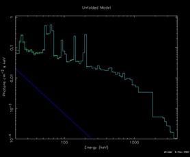 |
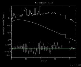
Note that without the "setplot group" command, XSPEC would plot 19 sets of spectral data, models and residuals. The can become confusing, especially as the number of spectra included in an analysis becomes much larger than 19! On the other hand, it can be useful to divide the data into subsets for plotting purposes, e.g. setplot group 1-6 7-12 13-19, to get an idea of relative shadowing effects of the coded-mask. The left hand plot illustrates the source model, the background model, the total model (i.e. source + background), and the data (here in count rates per channel). The right hand plot illustrates the "unfolded model" (blue, power-law curve), the summed model, and the data as a photon flux. A possible source of confusion is the similarity of the background model curves plotted in theses two separate representations. The explanation is that the background, which is dominated by instrumental contributions, is modeled in detector count space (i.e. the background response matrix has unit effective area. Thus, to be strictly correct, the right-hand plot is a hybrid of the photon source model and the detector-rate background model. We further note that at the present time, XSPEC does not have the capability to plot (or store and manipulate) the background subtracted data. This is a feature under consideration for a future release.
If we had chosen a observation containing more than a single source, the procedure would have been similar, except that the sequence of model commands would be extended, e.g.
XSPEC12>data ./MyDataDir/GCDE_aug_03.pha{1-475}
…
XSPEC12> model 1:1e1740 po
…
XSPEC12> model 2:gx1_4 po
…
XSPEC12> model 3:bkg spibkg_lo
…
Here data from the Galactic Center deep exposure campaign were loaded, and two sources are sought. In this case, a much larger number of spectra were loaded (475 spectra corresponds to one full 5´5 dither using all 19 detectors.
In this case, the simple approach of applying constant background (i.e. no detector-to-detector or pointing-to-pointing variation) to the full data set is likely to be a poor approximation. A more realistic approach would be to use the XSPEC grouping capability to handle such variations in the background solution. This can be accomplished in the usual manner (refer to the description of the grouping command in this document), however, it can become tedious in terms of the required command line inputs. For example, to establish a separate data group for each detector for a long (e.g. 5´5 dither) observations, a sequence of commands such as this would be required:
XSPEC12> data 1:1 ./MyDataDir/rev0044_Crab.pha.fits{1}
XSPEC12> data 2:2 ./MyDataDir/rev0044_Crab.pha.fits{2}
XSPEC12> data 3:3 ./MyDataDir/rev0044_Crab.pha.fits{3}
...
XSPEC12> data 19:19 ./MyDataDir/rev0044_Crab.pha.fits{19}
XSPEC12> data 1:20 ./MyDataDir/rev0044_Crab.pha.fits{20}
XSPEC12> data 2:21 ./MyDataDir/rev0044_Crab.pha.fits{21}
XSPEC12> data 3:22 ./MyDataDir/rev0044_Crab.pha.fits{22}
...
XSPEC12> data 19:38 ./MyDataDir/rev0044_Crab.pha.fits{38}
XSPEC12> data 1:39 /MyDataDir/rev0044_Crab.pha.fits{39}
XSPEC12> data 2:40 ./MyDataDir/rev0044_Crab.pha.fits{40}
XSPEC12> data 3:41 ./MyDataDir/rev0044_Crab.pha.fits{41}
...
XSPEC12> data 18:474 ./MyDataDir/rev0044_Crab.pha.fits{474}
XSPEC12> data 19:475 ./MyDataDir/rev0044_Crab.pha.fits{475}
One might then for example, make a first cut attempt by fitting a constant background. Then, as a next step, one might allow the normalization terms of the background model to vary over the groups (i.e. over the detector plane). This is accomplished with the "untie" command, using the following sequence:
XSPEC12> untie bkg:52
XSPEC12> untie bkg:78
XSPEC12> untie bkg:104
XSPEC12> untie bkg:130
XSPEC12> untie bkg:156
XSPEC12> untie bkg:182
XSPEC12> untie bkg:208
XSPEC12> untie bkg:234
XSPEC12> untie bkg:260
XSPEC12> untie bkg:286
XSPEC12> untie bkg:312
XSPEC12> untie bkg:338
XSPEC12> untie bkg:364
XSPEC12> untie bkg:390
XSPEC12> untie bkg:416
XSPEC12> untie bkg:442
XSPEC12> untie bkg:468
XSPEC12> untie bkg:487
Note that use of the "bkg" identifier, which associates the parameters index with the background model. The specific sequence of numbers use here requires some explanation; the particular background model employed has 25 parameters (which simply correspond in rank order to the 25 most variable individual bins), and a normalization term, i.e. parameter 26. Thus, the normalization for the second detector group is parameter 52, for the third parameter 78, and so on. Similar command sequences can be used to untie additional background model parameters. Supposing that we did this and refitted the data. We then might, for example wish to go back and freeze the individual normalization terms with the freeze command:
XSPEC12> freeze bkg:26
XSPEC12> freeze bkg:52
…
XSPEC12> freeze bkg:487
By now though, you probably get the idea that this all requires an unreasonable amount of command-line input. To circumvent this problem, a number of INTEGRAL/SPI specific "tcl" scripts are available which greatly streamline this process.
INTEGRAL Specific Command Line Scripts
SPIdata
The SPIdata procedure, which when installed can be treated as an XSPEC command, greatly facilitates the data initialization step. For example, the command
XSPEC12> SPIdata ./MyData/Dir/rev0044_crab.pha 475 det Y
Opens the Crab observation spectral data file, reads the 475 spectra into memory, grouping them by detector. The "Y" then indicates that, yes, I wish to ignore the spectral data channels corresponding to the known detector-electronic noise contamination (this is the default). Instead of "det" as the grouping option I could have selected "time" to group by time (quantized into dither-pointing intervals). A "-" lead to the data being initialzed into a single group. The command:
XSPEC12> SPIdata ./MyData/Dir/rev0044_crab.pha 475
Reads the 475 spectra into a single data group, and ignores the undesirable channels. If you forget all this, the command
XSPEC12> SPIdata -h
will remind you. The scripts SPIuntie, and SPIfreeze have similar command-line syntax.
SPIuntie and SPIfreeze
XSPEC12> SPIuntie bkg 475 19 -1
The SPIuntie command script will accomplish the same result as the sequence of "untie" commands in the INTEGRAL/SPI example presented in this document. In that case, we had loaded 475 spectra associated with a single 5´5-dither pattern centered on the Crab nebula. The spectra were grouped by detector, which is a common approach to SPI analysis given the known detector-to-detector variations in the background rates. Suppose after an initial fitting pass, for which we assumed a single background spectrum, we know wish to untie the individual data group (i.e. detector) background models. This can be accomplished by issuing 25 "untie" commands as previously noted, or in a single command line using the SPIuntie command:
XSPEC12> SPIuntie bkg 475 19 -1
untie bkg:52
Chi-Squared = 1.2030200E+04 using 1615 PHA bins.
Reduced chi-squared = 7.5852458E+00 for 1586 degrees of freedom
Null hypothesis probability = 0.0000000E+00
untie bkg:78
Chi-Squared = 1.2030200E+04 using 1615 PHA bins.
Reduced chi-squared = 7.5900314E+00 for 1585 degrees of freedom
Null hypothesis probability = 0.0000000E+00
untie bkg:104
renorm: no renormalization necessary
Chi-Squared = 1.2030200E+04 using 1615 PHA bins.
Reduced chi-squared = 7.5948231E+00 for 1584 degrees of freedom
Null hypothesis probability = 0.0000000E+00
…
One might then make a second pass at fitting the data, hopefully leading to improved statistics. Subsequently, additional background model parameters could be untied using the SPIuntie procedure as well. For example, to untie three additional parameters over the full data set[1], the command syntax is:
XSPEC12> SPIuntie bkg 475 19 1 3
…
This will untie the first 3 parameters of the background model identified by "bkg", i.e. equivalent to issuing (475-1)´3 individual untie commands. Note that you can always be reminded of the command-line argument definitions by typing "SPIuntie -h" at the XSPEC prompt.
Suppose now that you are satisfied with the relative background normalization terms, and wish to freeze them at their current values for subsequent fitting passes. This could be accomplished using the SPIfreeze command script:
XSPEC12> SPIfreeze bkg 475 -1
XSPEC12>SPIfreeze bkg 19 1 -1
freeze bkg:52 1
Chi-Squared = 6.6232600E+05 using 1805 PHA bins.
Reduced chi-squared = 3.7589444E+02 for 1762 degrees of freedom
Null hypothesis probability = 0.0000000E+00
freeze bkg:78
Chi-Squared = 6.5791894E+05 using 1805 PHA bins.
Reduced chi-squared = 3.7318148E+02 for 1763 degrees of freedom
Null hypothesis probability = 0.0000000E+00
…
As with the SPIuntie command script, typing "SPIfreeze -h" at the XSPEC prompt will scroll the command-line definitions to your screen.
[1] Note that the current SPI background models, which are documented elsewhere, are designed so that the parameter list is hierarchically ordered in terms of decreasing criticality. Thus, freeing the first parameter is likely to have the most significant impact on the statistics, the second parameter, the next most significant, and so on.